Cycles/EEVEE Improvements - Weekly Reports

Week 1: May 27 - 30

  • Added more operations to the Vector Math node and implemented dynamic inputs. [Ba52006]
  • Implemented dynamic inputs to the Math node. [Bfac13b]
  • Changed the default Vector Socket drawing method. Introduced Compact Sockets. [B18be4b]

Week 2: May 31 - June 7

  • Added dynamic inputs to the Mapping node. [Bab1817]
  • Added Map Range node. [B6e3ae3]
  • Added Clamp node. [B1b7a46]
  • Started writing Developer Documentation.

Week 3: June 7 - 14

  • Published Developer Documentation on Adding Cycles Nodes. A work in progress for the entirety of GSoC. [link]
  • Refactored hashing code and implemented White Noise node. Implemented using Jenkins’ lookup3 hash for compatibility with OSL. [B167d87]
  • Worked on refactoring and improving the Voronoi texture.

Week 4: June 14 - 21

Week 5: June 21 - 28

  • Worked on completing and refactoring the voronoi node.
  • Add 1D, 2D, and 4D versions of perlin noise. [B931da1] [Be7f7b9]
  • Simplify socket availability update code. [Bc73a56]
  • Corrected handling of unavailable sockets in Node Wrangler. [D5123]

Week 6: June 28 - July 5

  • Completed the 1D, 2D, and 4D versions of perlin noise.[B100772]
  • Add 1D, 2D, and 4D versions of musgrave texture. [Bc63491]

Week 7: July 5 - 12

Week 8: June 12 - 19

  • Added Volume Info node. Provides Color, Density, Flame, and Temprature of smoke objects. [B6fef86]
  • Added Vertex Color node. [Bef1e09]
  • Added Object Color to Object Info node. [B293bac]
  • Added Alpha output to Vertex Color Node. [Bf06620]

Week 9: June 19 - 26

  • Added Alpha output to Vertex Color Node. (SVM and OSL) [Bcd1351]
  • Started working on Spline Info node. Still don’t understand how the code base works, so we are no where near an implementation yet.

Week 10: June 26 - 2

  • The first half of this week was spent working on the Spline Info node. Unfortunately, I couldn’t finish an implementation in a timely manner.
  • The second half of this week was spent on refactoring code, cleaning up code, fixing bugs, optimization, handling backward compatibility, and writing versioning code.

Week 11: June 2 - 9

  • This week was spent on refactoring code, cleaning up code, fixing bugs, optimization, handling backward compatibility, and writing versioning code.

Week 12: June 9 - 16

28 Likes

This post provide an overview and examples of the features that have already been implemented.

Vector Socket

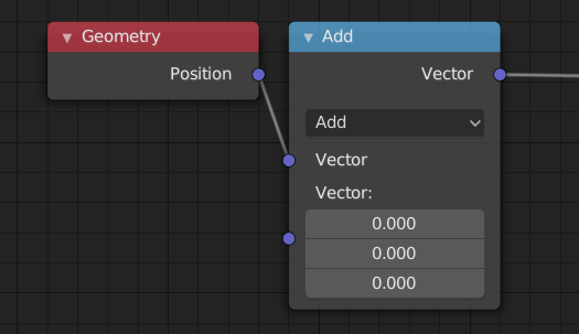
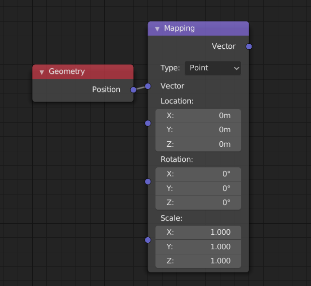
The vector socket is now drawn using a column layout by default:

column_layout

Vector Math

A multitude of new vector math operations have been added, including:

  • Entrywise Multiplication, Division, Floor, Modulo, Absolute, Maximum, and Minimum.
  • Vector Reflection and Projection.
  • Vector Scalar Multiplication, Length, and Distance.

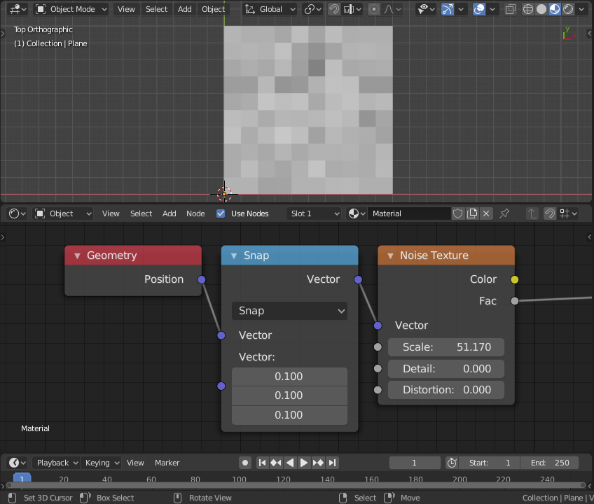
Snapping, for instance, can be used to easily create cell noise:

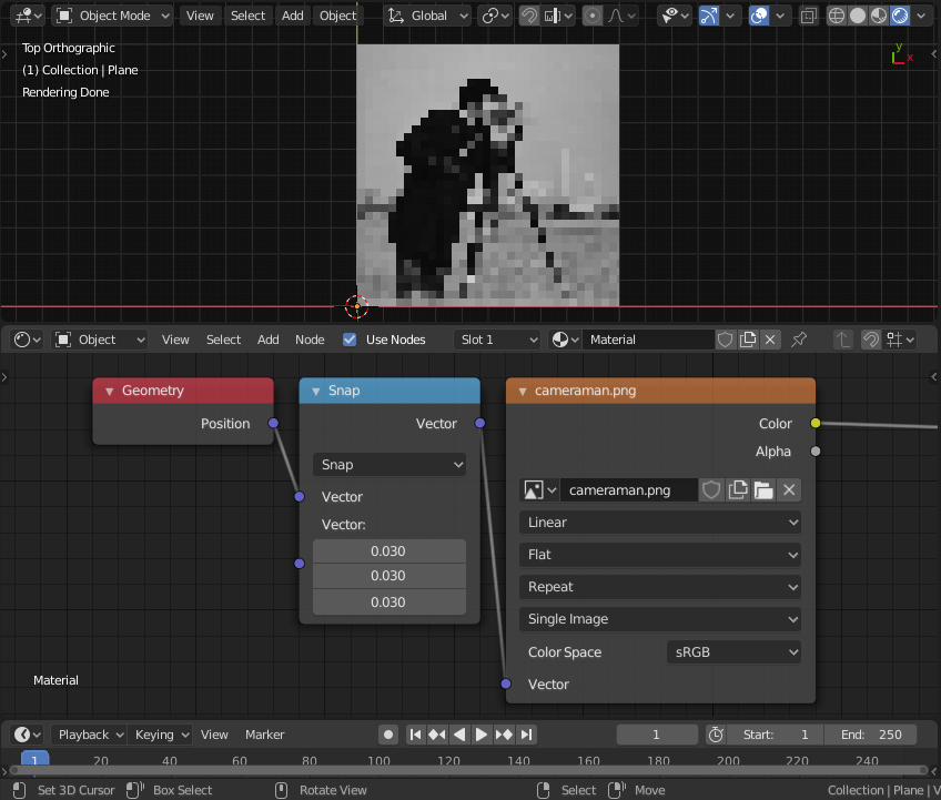
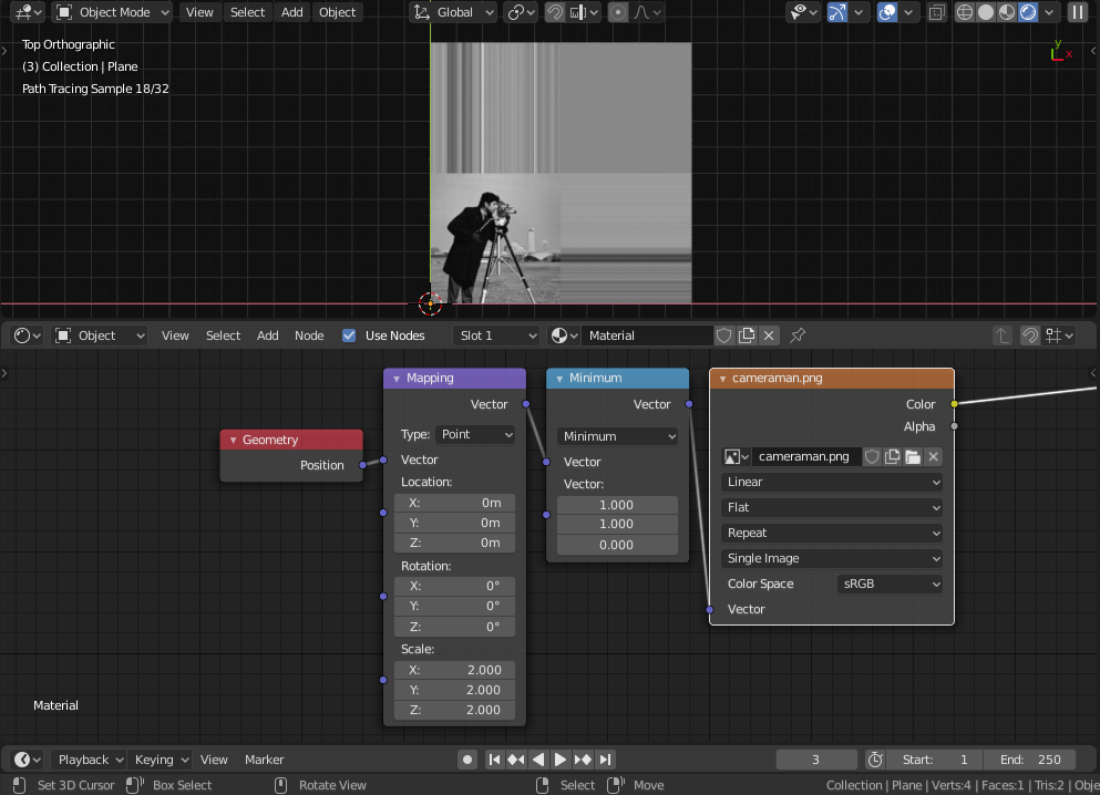
Or it can be used to easily resample images through quantization of space:

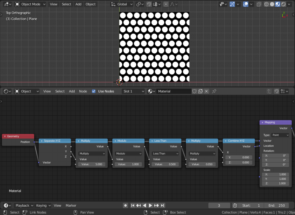
Modulo can be used to repeat patterns, for instance, creating a dot pattern:

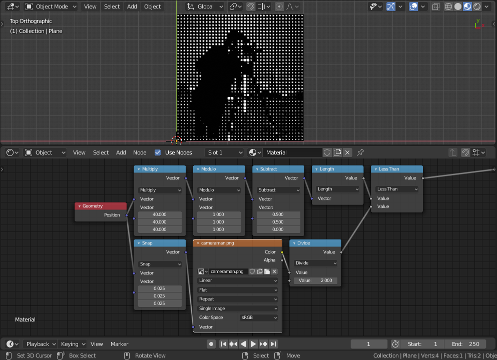
Modulo and Snap, together, can be used to create a stippling pattern:

Mapping Node

The mapping node is now dynamic, taking variable inputs:

For instance, given the following radial pattern:

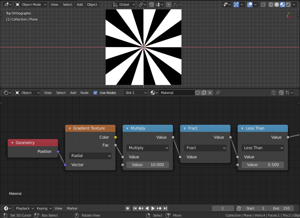
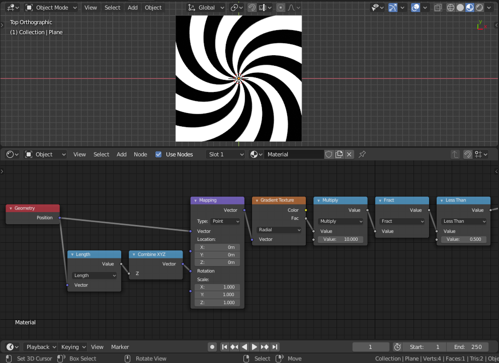
We can deform the pattern by rotating the space based on the distance to the origin as follows:

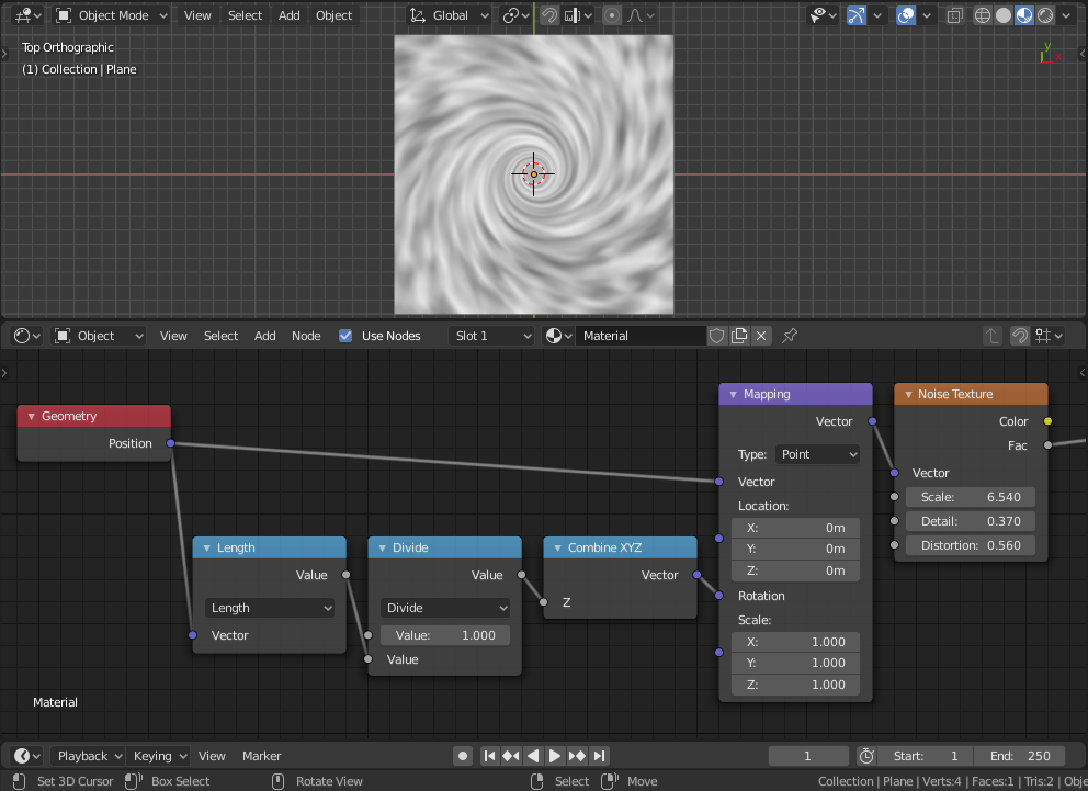
Or we can evaluate a noise at this space to get a vortex texture:

We can also achieve shearing through variable translation as follows:

Or we can shift the previously created dots in an alternating pattern as follows:

The max and min options have been moved outside of the node to the max and min operations of the Vector Math node:

Map Range

A map range node similar to that of the compositor’s was added:

Clamp Node

A clamp node was added to replace the math clamp option:

64 Likes

Holy Moly man, amazing work looks really promissing!
Keep at it!

3 Likes

This so exciting!! Seeing awesome devs like you working on Blender, creating cool tools like this gives me so much hope!

4 Likes

That’s awesome! Keep up the paste! Very cool! I’ve been waiting for this mapping node for years

1 Like

Really cool stuff ! However I think Map Range default “To min” and “To max” could be 0 and 1 as we more often need to normalize the input

Thanks! Those are already the defaults. The above screenshot is just an example.

2 Likes

Amazing opportunities for procedural texturing! Keep it grow))

Absolutely fantastic. Thank you.

Great work! Thank you!

Seriously, thanks so much! The clamp node alone will make things a lot easier to control!

1 Like

Awesome! I am especially excited for the Remapping node, that is a huge quality of life improvement.

1 Like

Fantastic!!! … Good Job.

White Noise

A new White Noise node was added. The node can operate in 1D, 2D, 3D, or 4D space.

Voronoi Texture

The voronoi node was rewritten to support much more modes of operation. Each of the following sections describe one of those modes of operations.

Dimensions

The node can now operate in 1D, 2D, 3D, or 4D space.

1D

One dimensional voronoi can be used, for instance, to create a brick texture with random width:

2D

Two dimensional voronoi can be used to create a somewhat accurate 2-distances to voronoi cells. Something that was otherwise hard/impossible to get with 3D voronoi. This can be used to create cracks with uniform width:

3D

We already had 3D voronoi before, so nothing was added here.

4D

Four dimensional voronoi can be used to animate voronoi in 3D space. In other words, the fourth dimension can be a function of time:

Or it can be used create a loopable animated voronoi in 2D space. This gif loops!

Jitter

The new jitter input controls the uniformity of the voronoi cells:

Features

In general, we fixed some symmetry issues and improved precision. The node lets you select what voronoi feature you want to compute. The following features are supported.

F1

This is the standard F1 feature we had before. However, we now provide the position of the voronoi cell as an output:

The position can be used to compute local texture coordinates in voronoi cells as follows:

The significance of this local texture coordinates will become apparent later.

Smooth F1

Voronoi can’t be used in organic textures due to the hard discontinuities at the cell edges. For that reason, we introduced a smoothed voronoi textures. A comparison between normal F1 distance and smoothed F1 distance is shown below:

The smoothness is more apparent if the node was used as a displacement texture. Both of the following textures are smooth with different smoothness values:

The ID color of the voronoi cells is also smoothed, introducing a new type of noise. Different smoothness values are shown below:

In fact, it is just a Value Noise:

Yes, we just got Value Noise free of charge. The cell position is also smoothed:

Such smoothness can be utilized to create all sorts of patterns. The difference between smoothed F1 and F1, for instance, can be used to create a beveled voronoi cell pattern:

A high smoothness value with color based masking can produce a water droplets texture:

The isolines of the smoothed distance is meta-ball like:

F2

This is just the standard F2 we had before. The primary purpose of F2 is to compute the well known F2-F1 pattern for non-euclidean distance voronoi:

F3 and F4

F3 and F4 were deprecated.

Distance To Edge

This is mode of operation computes the distance to the voronoi cells edges. This is a much more accurate version of the cracks feature we had before, which was an F2-F1 algorithm.

Only euclidean distance is supported for now. Manhatten and Chebyshev distances may be supported in the future while Minkowski will not be considered.

N-Sphere Radius

This mode of operation computes the radius of the n-sphere inscribed in the voronoi cells. In other words, it is half the distance between the closest point and the point closest to it. Consequently, it is the max radius of the bounding n-sphere that each cell is allowed to have to avoid intersection.

The simplest example would be as follows. Notice how the n-spheres never intersect:

A more practical example would be:

We can use this setup to create a very robust and highly efficient scatter node, which I shall show now. We are going to use the local coordinates we previously computed:

And we are going to scale the local coordinates based on the n-sphere radius and rotate it based on the cell color along the z axis. Finally, we are going to evaluate the required texture to scatter at this texture coordinates:

And voila, we just created a scatter node! Here is 3D sphere packing:

76 Likes

Ok. That’s good enough. You can stop now.

4 Likes

Omar, thank you for these detailed breakdowns of whats been added. It’s fantastic to have the pictures as visuals for what your talking about! As always, thank you for your work. It’s turning out so well I feels like a dream.

3 Likes

Don’t listen to him!

More! More! :grin:

9 Likes

wow, can’t wait to see users experimenting with new interactive demos

1 Like

The new nodes look great. I would very much appreciate included node setup presets for non-math people like me.

Please use this thread for feedback:

5 Likes