Closures and Bundles are new concepts in Geometry Nodes that have recently been added to the main branch as an experimental feature. You can read more about the basic idea in the pull request #128340 or the workshop blogpost. In this post i want to explore how closures can be used to implement emitters for particle systems as a way to establish best practices and maybe find shortcomings that need to be addressed in the future.
Blend file: emitter-closures.blend
Important:
- Use a recent build that has the closures-and-bundles feature (4. April or later).
- Enable the “Bundle and Closure Nodes” feature in Preferences > Experimental > New Features
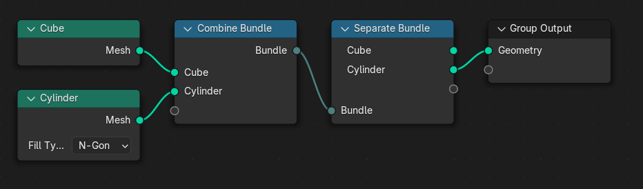
Bundle
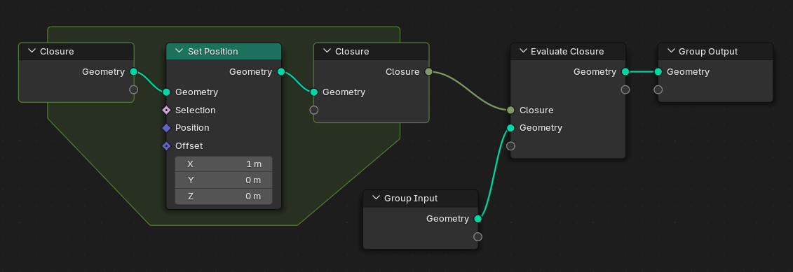
Closure
A particle system typically starts out empty and then uses one or more emitters to generate particles and insert them into the system. The emitter only defines the initial location, velocity, and other properties of particles. Afterwards any new particles are released and simulated alongside existing particles using physics, collision, or any number of other features. I won’t go into detail about these other particle system components here to keep the post focused.
Since there are many different possible types of emitters and many ways in which users may want to customize them it’s virtually impossible to make a particle system node group that satisfies all needs. Take the existing particle system implementation in Blender: It implements a wide range of particle distribution methods and customization with textures, and yet still becomes insufficient for all but the simplest cases. The wide range of possible feature combinations makes it hard to test and maintain, and some combinations of settings (e.g. anything involving rotations) are known to fail more often than not.
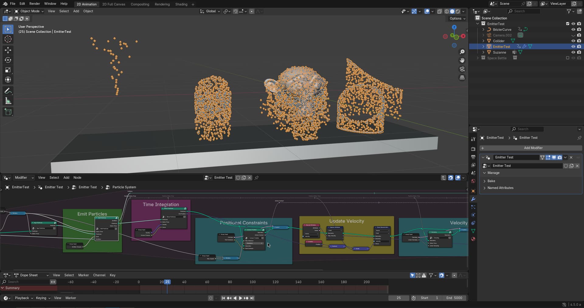
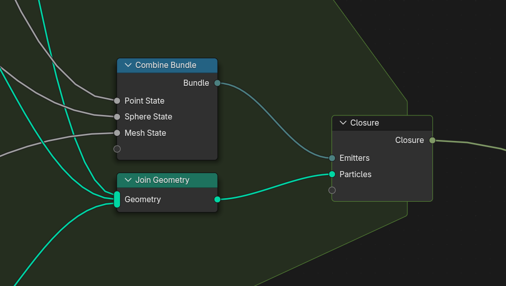
In my test scenario i’ve implemented a fairly standard physics-based particle system with basic movement, collision, and forces. Particles pass through a number of stages in each time step, the first of which is to generate new particles and combine them with existing ones. In a conventional node setup this would require a user to modify the primary simulation node asset and insert their own nodes. Instead, i’m now using an Evaluate Closure node to delegate particle emission to an external closure. This closure outputs a set of points, which are joined with the existing particles.
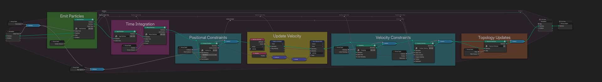
Particle system stages
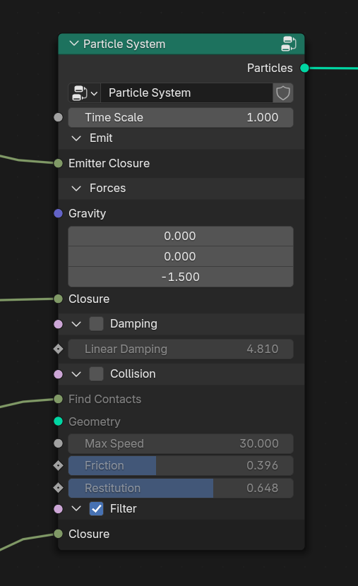
Particle system node from the outside
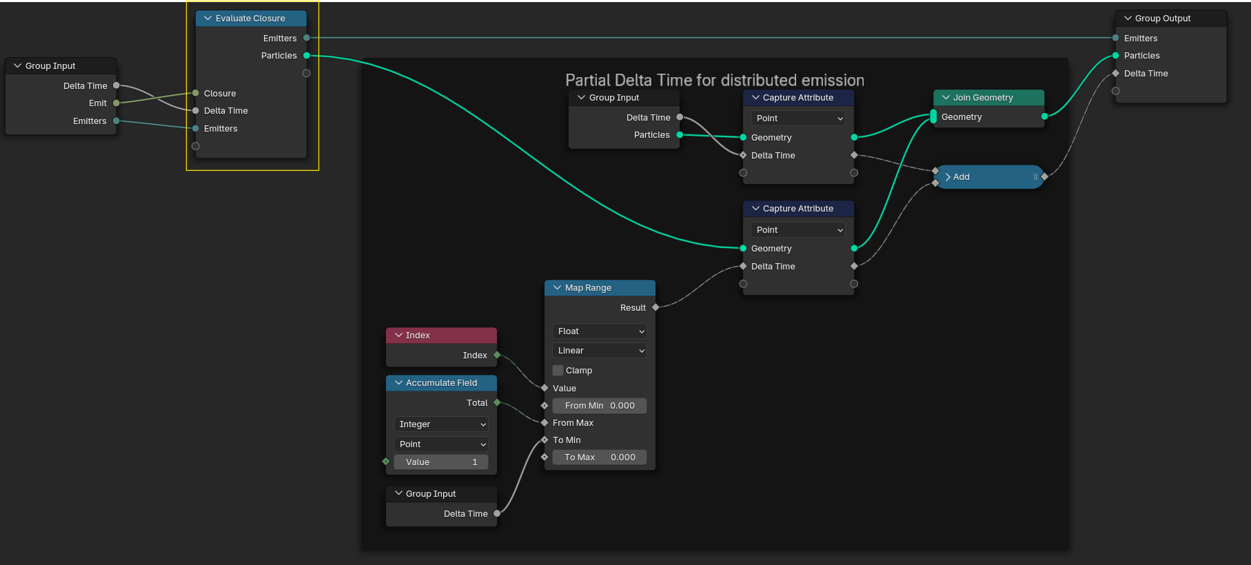
Evaluating the emitter closure
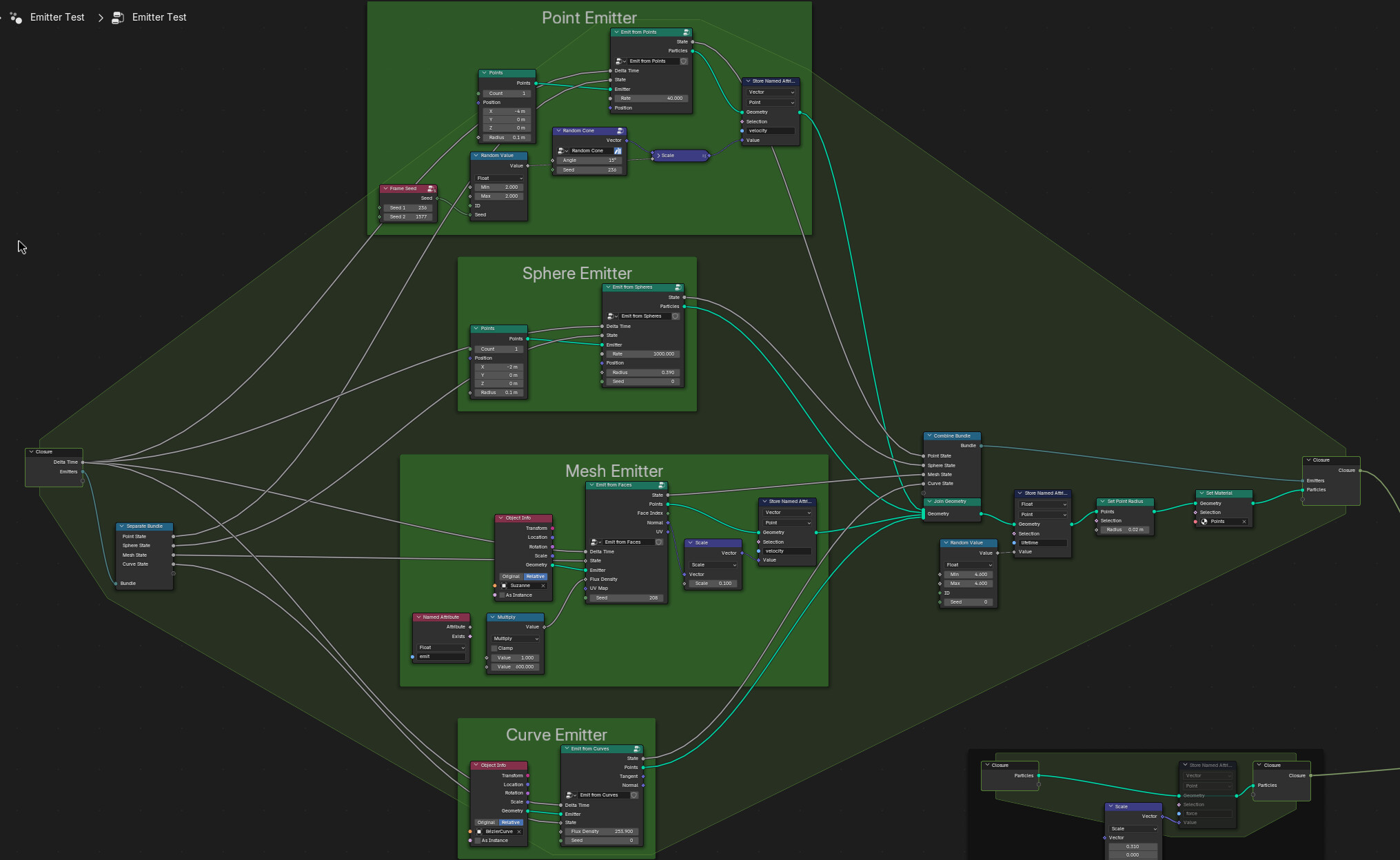
Big closure with multiple emitters
The inputs and outputs of a closure must match the expected inputs and outputs at the point of evaluation. This needs to be communicated outside of the node setup itself in some way. While there is some basic feedback about missing sockets, knowing upfront what an emitter closure should do is important. Templates and example implementations can help, but some other way of documenting the closure “contract” would be helpful in the future.
Point Emitter
One of the simplest emitter types is a point emitter. Particles spawn at a single point in space. This point can remain fixed, or it can be animated over time.
Values in a closure, such as the emitter position, can be animated either by directly animating node properties (preferably through modifier buttons) or by animating an object and reading from an Object Info node.
The number of particles emitted can be defined in different ways:
- Burst: A fixed number of particles is emitted at a specific point in time.
- Rate: The amount of particles emitted depends on the time step size. The rate can change over time.
With rate-based emission a naive implementation might simply multiply the rate by the time step size and output this amount of particles. However, if this amount is less than 1, no particle would ever be emitted! Any fractional amount of emission would also be ignored, leading to an actual emission rate that is smaller than the nominal rate.
To fix this, the emitter should add up the fractional amount of particles emitted, so that any time the accumulated amount crosses an integer value a particle gets emitted. This way even very low emission rates are possible, spawning a particle only every couple of seconds or so.
Left side: Low emission rate leads to cutoff below 24 (less than 1 particle per frame)
Right side: Cumulative emission count supports arbitrarily low emission rates
Keeping track of emitter state requires some extra data input/output. The closure itself cannot store the emitter state, so the particle system has to store this state information instead. It can store a generic Bundle for all emitter state data, and the closure then reads the necessary value for each emitter from the bundle. The closure returns the modified emitter bundle and the simulation stores it for the next iteration.
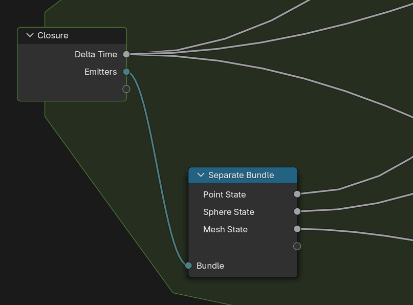
Read state for various emitters
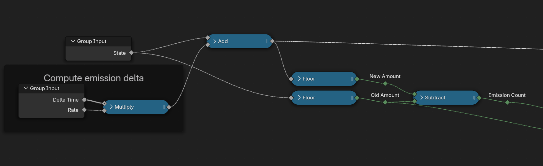
Add emission to the state
Write state to bundle
Sphere Emitter and Other Shapes
Only a small change is needed to go from point emitters to sphere emitters and similar geometric shapes. Instead of placing each new particle at the same point, we now randomly distribute particles on the surface of a sphere.
The math for chosing a point on a sphere at random won’t be derived in detail here, suffice to say that a uniform density on a sphere can be achieved by picking a uniform z coordinate in [-1..1] range, radius r = \sqrt{1 - z^2}, and rotation around Z by a random angle. Other geometry primitives such as cylinders, cones, etc. have their own methods for uniform random distributions.
In order to change the random position for every new particle we have to make sure that the ID value for each particle is unique. The “local” index of the new particles will always start at zero, so the randomized positions would also be the same for each new batch of particles. To avoid this we need to assigne a unique ID to each new particle, which the Random utility nodes can use. A simple way to compute a unique ID is to take the “local” index and add the cumulative emission count. The Seed value can also be varied for each emitter to give it a unique distribution.
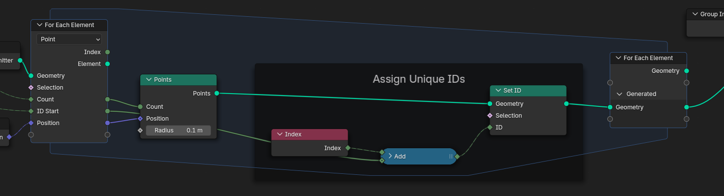
Unique ID for each particle
Mesh Emitter
A mesh emitter places particles at random locations on the mesh surface. The density of particles should be uniform by default, with an optional factor that can be used to limit emission to certain areas, for example by painting an emission map or a vertex attribute.
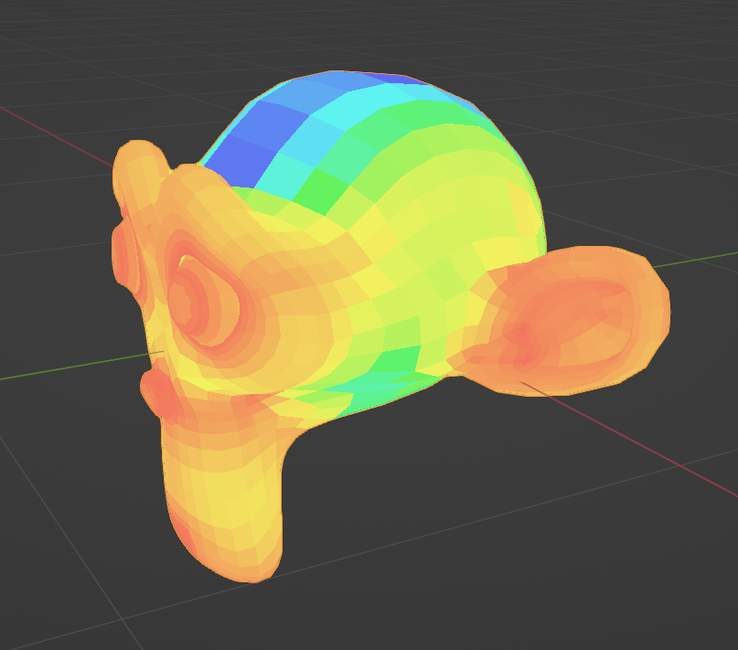
Varying face area on Suzanne
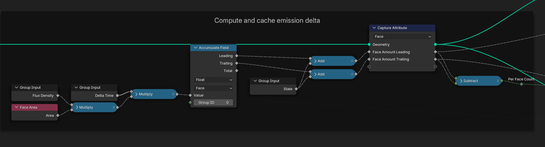
Cumulative emission amounts
The overall amount of particles to emit in a single time step is determined by integrating the density over the entire mesh surface. This can be approximated by linear interpolation in each face and a sum over all faces. Since sampling general Ngons is hard, the mesh is first triangulated to simplify the problem. It should be noted that the total emission count is the only value necessary to remember from previous iterations, it is not necessary to store a count per triangle.
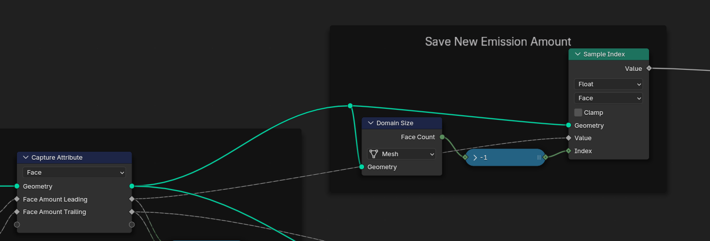
Total amount is the new emitter state
Chosing a specific mesh face with varying probability would require evaluating the quantile function of the distribution, which is difficult. An easier approach is to determine the amount of emission for each triangle separately, and then generate the required number of particles on each triangle. The emission count is accumulated over all triangles so that particles are distributed over the whole surface. Starting at the total count of the previous frame, like we did for point emitters, ensures a steady increment at low rates. Additionally shuffling the order of mesh faces avoids emitting particles in the same locations every time.
Once the actual integer amount of particles for each face in a time step is computed, a For Each Element zone is used to generate per-triangle points. Attributes for each triangle point, including the position, are interpolated between the three corners of the triangle. A set of 3 barycentric weights is computed and each attribute is mixed using these factors. In the current implementation the weights are chosen uniformly, leading to a “flat” distribution across the face. This is fine for relatively dense meshes, but if actual density interpolation on each triangle is necessary a different technique could be used (e.g. J. Portsmouth, “Efficient barycentric point sampling on meshes”, 2017). As an additional optimization, the corner attribute vectors are packed into a single matrix attribute, which can be interpolated with a single vector transformation (reduces number of sockets by factor 3).
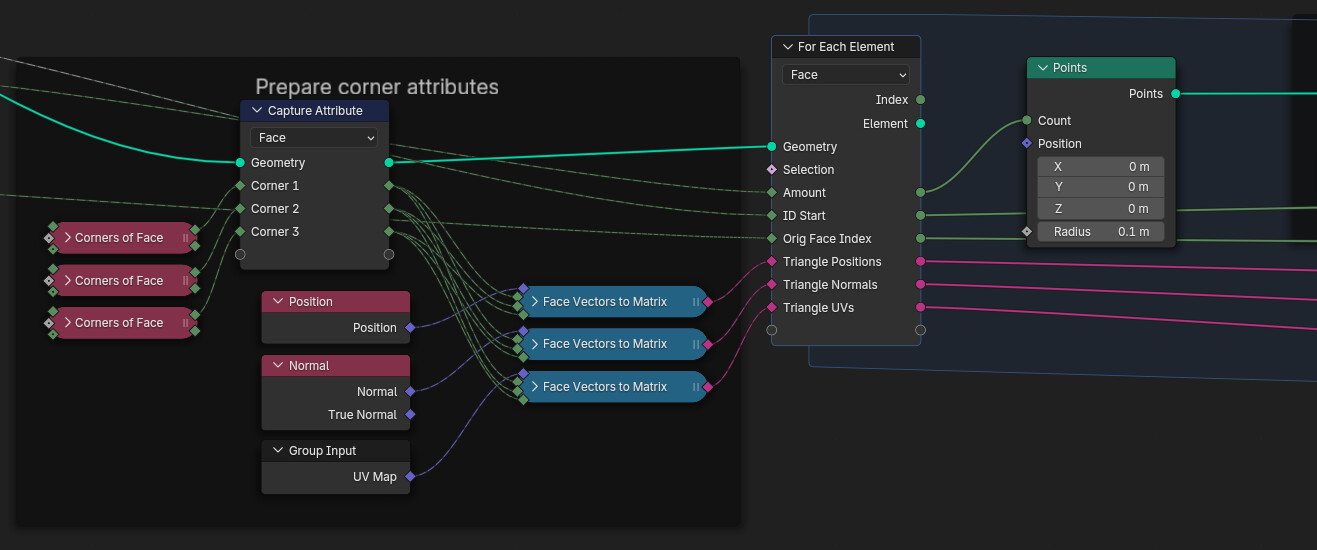
Using a For-Each zone to generate particles
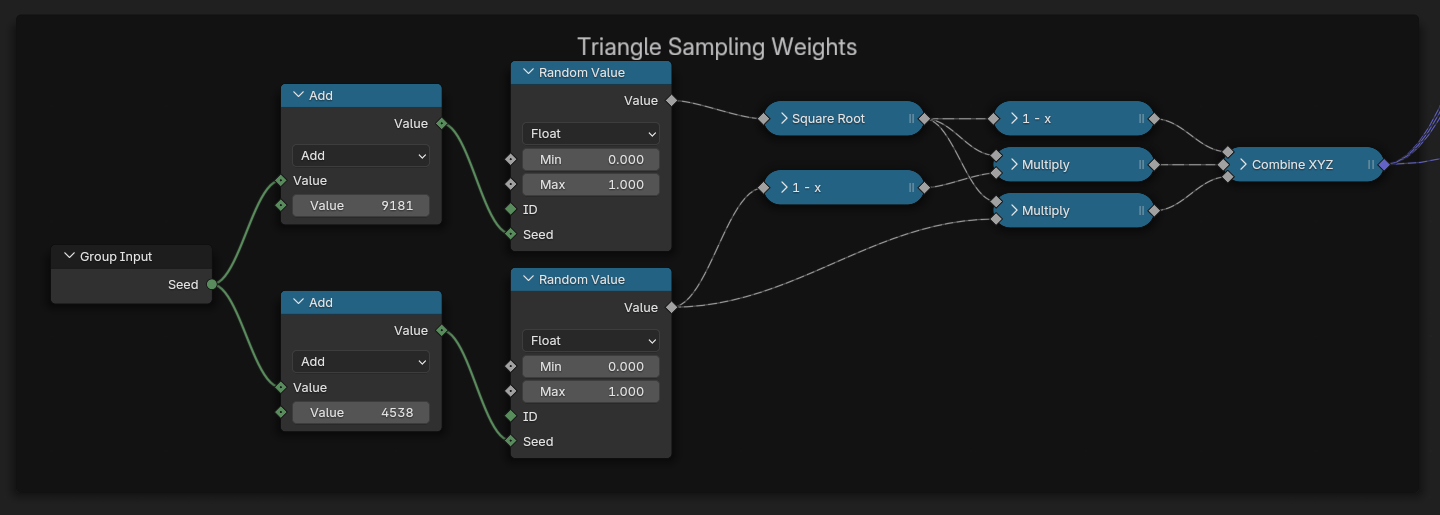
Sample weights for a triangle point
Curve emitter
Similar to a mesh emitter, on a curve emitter the density can be variable. To enable efficient sampling the curve is first converted into a series of simple linear segments, equivalent to triangulating a surface mesh. The “evaluated” curve points are the natural choice for this.
Shuffling curve segments is not possible directly because the curve has a fixed order of points, but this can be circumvented by converting the curve to a point cloud first. Each point represents a small linear curve segment. Any attributes we may need later, such as the curve normal direction, must be captured before conversion.
Similar to mesh sampling, each segment generates a number of points according to its density factor. Two weights are chosen and the attributes of the vertices are interpolated.
Conclusion
The good stuff:
- You can now customize behavior of complex node-based assets without having to modify the original asset.
- Only necessary features need to be made available. Node asset UI remains lean instead of providing mostly-unused buttons for every possible scenario.
- Users can choose between different implementations and balance performance, capabilities, and complexity based on individual needs.
However, they also still have some rough corners and can add more complexity:
- Closures require a clearly documented signature of inputs and outputs. Templates or example implementations can help with that, but better support in the asset system may be required for those.
- Currently a closure must always be defined, otherwise the evaluation produces no output. Having a default “pass-through” implementation or a boolean socket to indicate a “null” closure on evaluation would make sure the system works out-of-the-box without having to set up dummy closures.
Note: With upcoming field support it won’t be necessary to store named attributes as often. An empty field yielding zeroes will often be sufficient as a “default” implementation. - Combining multiple emitters requires manually separating and re-combining data in a single closure. Future support for lists could make this more user-friendly. Implementing a quasi-list with a closure is also feasible, but increases the complexity significantly.
- Having to pass around extra bundles for storage can make things complicated. It’s up to users to make sure the right geometry is passed to a given emitter.
Note: I’ve tested putting a simulation zone into a closure to cache state internally, but this is unsupported.
Note 2: It may be possible to put both the closure and supplemental data in the same bundle to only have a single socket, but bundles with closures don’t currently work in simulation zones.
Closures are a valuable addition to geometry nodes. Currently they are a tool for technical users more than artists, but they should become more accessible over time. I hope this initial set of emitters can grow into a truly node-based particle system in the future.