Fit bezier curve to mesh

[floka]

Hi,
is there a oprtion via python to fit a curve (bezier) to mesh?
Blender has already a cruve fit algorithm (i guess - curve decimate) but is this algorithm accessable via python ?.

[Josephbburg]

What do you mean by “fit a curve to mesh”? Please explain the before/after that you want.

[floka]

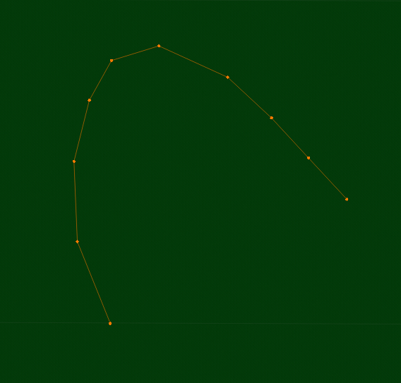
before:
There are a set of points from a mesh

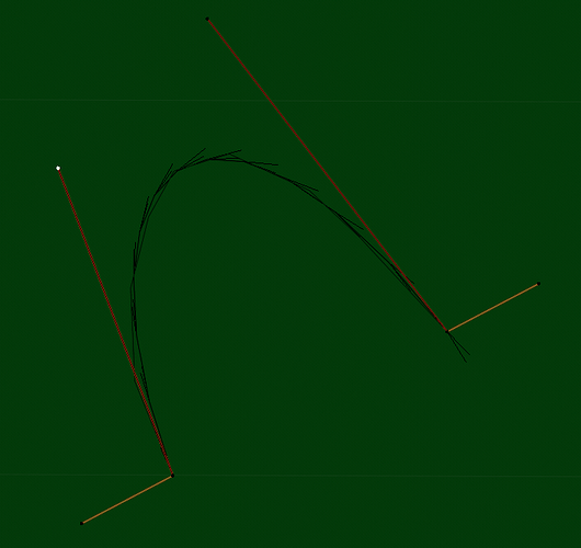
after:
A Bezier segment where the curve fits the point position.

There is a function to get the interpolated bezier points

 mathutils.geometry.interpolate_bezier(knot1, handle1, handle2, knot2, resolution)

but i need the reverse behaviour wehere you have the start and endpoint and also the interpolated points and get the handle vectors.

I hope that make sense.

[Josephbburg]

Thanks, that helps me answer you. Well, there is a library that you can easily build and import that was written by a Blender developer for, IIRC, internal use with the GP. It can import into Python. I haven’t tried it personally but I’ve been meaning to. I don’t know how portable it is, either. I’ve built it and imported it but I didn’t try to use it in my addon, because there was an easier, less precise way to do what I needed.

Within Blender, I don’t know of any curve fit function that’s exposed to the user, but I think internally it uses the library I linked for everything.

The easier, less precise way: Just make a Bezier curve from the points with all the control points set to ‘Auto’. There’s an operator for doing this already, and then I suppose you can use the curve-decimate addon (I don’t know how that one works).

[Josephbburg]

@floka

mathutils.geometry.interpolate_bezier(knot1, handle1, handle2, knot2, resolution)

I’ve found that this isn’t even a very helpful function. In my addon I convert the curve to a mesh and extract the data from it. It’s fast, reliable, and completely matches what the user expects. And it’s simple, too. Let Blender do the complex math!

Oh, also, this may be worth looking at: A Primer on Bézier Curves (thanks to @sybren for showing this to me )

[floka]

Thanks for all your help

[floka]

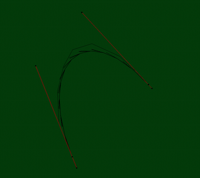
ok i tried the decimate option but the result is not so presice like in the curve fit library.
can you explain how i can use this library , do i have to compile blender?

[Josephbburg]

No you don’t have to compile Blender, just the library. I think it’s as simple as cloning the repo and make make install. But I haven’t done anything beyond building it, myself.

[grosgood]

@floka
Perhaps the experimental script at the end of this post can help you.
It employs numpy.linalg.lstsq to fit Bezier spline curves to stand-alone mesh edge loops.
The standalone mesh edge loops should themselves be products of conversions of curves to meshes.
I imagine that in a workflow, one would start with a curve and shape it to one’s needs, perhaps using a shrink modifier to profile the surface of another object. I suppose, while in edit mode, one could also copy out an edge loop of an existing mesh (‘Shift-D’), turn it into an independent mesh object (‘P’) then convert that mesh object into a curve. See Howto. For the terminally curious, Rainy Day Reading discusses the script’s design and limitations.

Caveat: This is not production code. It illustrates a use of numpy in Blender. Take care.

TL;DR

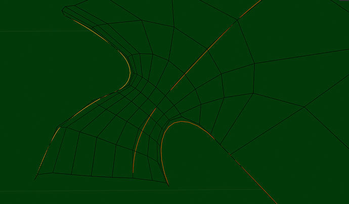
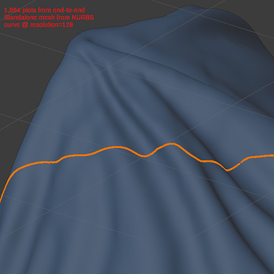
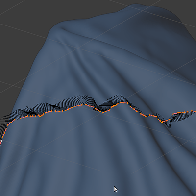
Dataset: A mesh generated from a curve (Object → Convert To → Mesh) Previously, the shrink-wrap modifier plastered the curve onto another mesh, blue in the illustration.

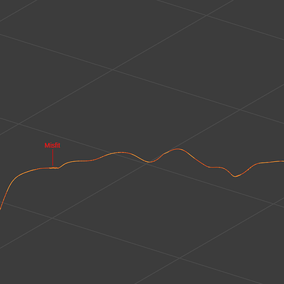
Fitted Bezier spline: Estimated using numpy.linalg.lstsq as a Least Squares solver.

Comparison: The estimated Bezier curve overlaying the mesh.

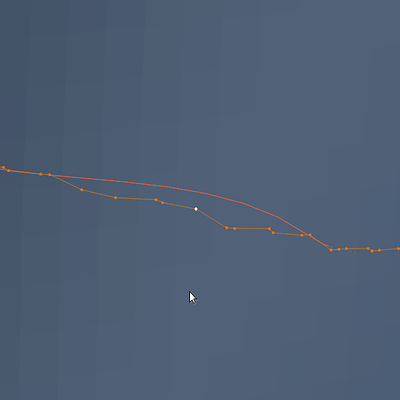
Misfits: Arise if there are irregularities in the mesh.
Howto:

1. Copy the script; paste it into a Blender text buffer.
2. Use any kind of Blender curve. Call it ‘Probe’ for discussion.

• Shape Probe or capture a shape with it - shrinkwraping Probe onto a surface, for example.

3. Convert Probe to a mesh - a free-standing edge loop.

• Caution: Don’t start with a mesh, bypassing Probe. See FIXME_1: in the script.
• If you DO copy out an edge loop from an existing mesh (Edit mode: Shift-D, P), creating a new mesh object, go to object mode, convert the new mesh object temporarily to a curve (Object → Convert To → Curve) then back to a mesh (Object → Convert To → Mesh).

4. Select the mesh-converted Probe; it should be the active object.
5. Run the script in the text buffer.
6. A fitted Bezier spline, ‘Fitted_Bezier,’ curve appears. It should closely track Probe.

• Adjust TOL in the script, making it bigger for more loosely fitting curves.

7. Use ‘Fitted_Bezier’ in your further modeling schemes.
8. Come some idle day, peruse Rainy Day Reading.

Rainy Day Reading

At it’s heart this script:

(1) makes explicit what is implicit in a very large number of ‘educated’ guesses we make, embodied in a matrix A - ‘educated’ in so far as we have a theory - a statistical model - with a few choice parameters x. This theory predicts how a large quantity of plot points b occur in the locations we’ve been given.

(2) tells us the liklihood of whether our theory is viable or a busted flush. If likely, then we have a solution with the x of Ax = b. That is, these x are very likely to be the correct control points for fitting a Bezier spline to the observed plot points constituting b.

What we don’t know: The explicit x - aka, our control points.

What we do know: An awful lot of locations b that - by gum! - look like a Bezier spline!

Our theory: A spline of cubic Bezier curves, each with a few choice parameters - their control points - can plot all the observed positions we have been given. Using just (a few) choice control points, we can predict other positions that could also be among the points we have been given.

Constructing our theory: For each spline segment, a cubic Bezier polynomial pairs a control point from x with a bezier basis function written in terms of an independent parameter u. Given u, the basis function returns a weight in the range [0…1] that weights the control point, establishing its contribution to a computed location. These basis functions are linked together in the sense that all the weights they compute add up to 100% - unity. Such things are called affine combinations. All the parts - contributions - make up a whole - the computed location in space. No more. No less. Otherwise the weights do not make an affine combination and the shape of the curve changes relative to its position with respect to the origin. Cubic polynomials have four terms, four pairings of control points with their allied basis functions. This weighted sum of control point locations constitutes one plotted point.

Relating the known to the unknown: A is a set of educated guesses produced by our theory. Each row of A connects a plot point from b to our theory through a set of weights, corresponding to each purported control point. Some people call A an observation matrix because of the way it connects observational reality (plot points) to theoretical fantasy (educated guesses). These weights set the contribution of purported control points drawn from x to the location of a specific plot point drawn from b. We don’t know where those purported control points are, but we provide hints in the form of implied behavior: wherever those control points are, when we weight their contributions - using these particular weights! - we compute the location of a corresponding plot point in b. Behind the scenes, we’ve used the Bezier basis functions by themselves to compute the weights. All of our myriad hints, one hint for each plot point, taken together imply a specific set of locations for the control points, or so we claim. For these hints are not grounded in any kind of reality. They are grounded in our theory, to wit: that a Bezier spline curve underlies this large list of locations. We are doing statistics here, not mathematics, and Bezier curves constitutes our statistical model.

Technique: Having composed our myriad educated guesses in A we ask a Least Squares Solver in numpy - numpy.linalg.lstsq to invert A and put on the right hand side of the equation, solving for the control points x. I’m not going into the LS technique here. I recommend Sec 15, Numerical Recipes in C, “Least Squares as a Maximum Likelihood Estimator” (Cambridge University Press, 2nd Ed. pp 657ff, Press, Teukolsky, Vetterling & Flannery). About a bazillion PDF’s of this reference are floating around the Web. While your nose is in that reference, also take a peek at Singular Value Decomposition (SVD), section 2.6, a technique to separate matrices like A into three, more computationally tractible matrices.

Bookkeeping: Most of it involves cooking up the guesswork matrix: A.

tryit() contains the development run-up to A culminating in the request to invert A and provide (1) likey coefficients (control points): x and (2) an array of residues in each coordinate of the plot point. These tell us if we have a busted flush in any one or more dimensions. The larger the residue, the more likely we have a busted theory.

1. plotpoints is a (very long) vector of plot points.

2. diff is a (one less long) vector of difference from one plot point to the next.

3. slen are those differences expressed as lengths, found by way of the Pythagorean Theorem.

4. ssum are the relative distances of each plot point from the origin of the purported curve. The first plot gets zero; the last plot gets one; the interior plots get a relative value, these derived from sums of lengths along the curve from the origin to the plot at hand (arc length), normalized by the entire length of the curve. These become trial u values, one proposed for each plot point in plotpoints.

5. obmx The observation matrix, aka A. There is a bit of numpy ufunc magic here. For example, bf0(ssum).reshape(ascol) applies the first basis function computation, elementwise, to ssum, producing a new array which is rotated into a column vector by the numpy array method reshape(). The four column vectors are then horizontally stacked into the observation matrix.

Main loop: Divide and conquer by binary division. We manage this through an array of slices kept in stack. Typical game: First try for the whole curve as one Bezier segment. If that theory exhibits high residue, then divide the plot point set by two and attempt to find fits for the two halves. And so on. When the stack empties, we have a sequence of solutions: in aggregate, the purported Bezier spline.

This is an illustrative script, not a production one. Script comments discuss a few weaknesses. I would be interested if people find areas where it works and where it does not, perhaps flushing out other weaknesses. Thank you in advance for that.

#! /usr/bin/python
"""Fit a Bezier spline curve to a standalone edge loop generated from
   a curve. For use with Blender 3D Python API. This code is for
   illustrative purposes only. It is not production-ready. Available
   under Creative Commons Attribution-NonCommercial-ShareAlike 3.0
   Unported License."""

import numpy            as np
import bpy
from bpy import data    as D
from bpy import context as C
from mathutils import Matrix, Vector

# In a production environment, these data should
# come from a user interface.
# Tolerance. Larger numbers give looser fits.
# TOL = 0.1    # This gives loose solutions - good for noisy data
# TOL = 0.01
# TOL = 0.001
# TOL = 0.0001
TOL = 0.00001  # This gives tight solutions - good for precision
RES = 8        # Sets mesh density for Blender curves.
NME = 'Fitted_Bezier' # Name of the fitted curve -
MINPTS = 4 # Don't fit slices smaller than four points.

# Lambdas for generating an observation matrix. These are
# Bezier basis functions which bakes in the idea that the
# observation data points lie along Bezier spline curves.
# Change these for other bases.
# ENHANCEMENT: Use Carl DeBoor's Algorithm instead of hard-
# wired basis functions.

bf0 = lambda u: u**3
bf1 = lambda u: 3*((u**2)*(1-u))
bf2 = lambda u: 3*(u*((1-u)**2))
bf3 = lambda u: (1-u)**3

def splitslice(stackslice):
    """From splice s return a list of two splices
       0: from beginning to mid-element,
       1: from mid-element to end"""

    interval = (stackslice.stop - stackslice.start) >> 1
    remainder = (stackslice.stop - stackslice.start) %  2
    return [ \
        slice(stackslice.start, stackslice.start + interval + remainder, 1), \
        slice(stackslice.start + interval, stackslice.stop, 1)              \
           ]

def tryfit(plotpoints):
    """plotpoints: numpy array of 3D space points. shape (N, 3)
       return: python list of numpy arrays, shape (4 x 3)
       Cubic Bezier spline control points."""

    dln = len(plotpoints)
    ascol = (dln, 1)
    diff = plotpoints[1:] - plotpoints[:-1]
    slen = np.array([np.sqrt((p**2.0).sum()) for p in diff])
    ssum = np.array([0.0] + [slen[:k].sum() for k in range(1, len(slen)+1)])/slen.sum()
    obmx = np.hstack(                               \
                      (                             \
                          bf0(ssum).reshape(ascol), \
                          bf1(ssum).reshape(ascol), \
                          bf2(ssum).reshape(ascol), \
                          bf3(ssum).reshape(ascol)  \
                      )                             \
                    )
    return np.linalg.lstsq(obmx, plotpoints, -1)

# Try to fit the whole dataset to a one-segment spline.
# If that fails, split and try halves. Recurse. Maintain a
# stack of to-do slices until the topmost slice on the
# stack fits. Pop it, save the fitted segment, and
# commence on the next slice on the stack. Recurse
# until the stack is empty.

aod = C.active_object.data

# FIXME_1: Generally, vertices read from a mesh data block aren't
# in any kind of order. vb assignment exploits the fact that an
# edge-loop generated from a curve 'happens-to-be' in geometric
# order. Replace this assignment below with an edge-loop-walker
# that reliably fetches vertices in geometric order - perhaps
# from a user-selected edge loop.

vb = np.array([v.co for v in aod.vertices])
stack = [slice(0, len(vb), 1)] # stack with one slice
sset = list() # Save set of fitted bezier curves

while bool(stack):
    # Residue furnishes per-dimension quality of fit
    # Larger residues indicate poorer fits. Not used -
    # rank: If less than 4, results not reliable
    # singular: As these approach zero, the corresponding
    #           control point contributes less to the solution.
    #           Small singulars suggest removing the
    #           corresponding control point from the
    #           solution.
    # tryfit should be in a try - except block to
    # catch fit failures.
    solution, residue, rank, singular = tryfit(vb[stack[-1]])
    ltol = np.sqrt((residue**2.0).sum())
    if (ltol < TOL) or (len(vb[stack[-1]]) < MINPTS):
        # Good fit - or slice too thin. Save
        # solution and pop the slice.
        stack.pop()
        sset.insert(0, solution)
    else:
        # Too much residue. Pop top slice,
        # divide it at mid-plotpoint and
        # make a list of left and right
        # slices.
        lslice = stack.pop()
        stack += splitslice(lslice)

# Construct Bezier curve data block from sset
DLEN = len(sset)
BINDX = 0
crv = D.curves.new(NME + '.Curve', type='CURVE')
crv.dimensions = '3D'
bseg = crv.splines.new('BEZIER')
bseg.bezier_points.add(DLEN)
bseg.resolution_u = RES
while bool(sset):
    dp = sset.pop()
    if not BINDX:
        # At start of Bezier curve spline
        bseg.bezier_points[BINDX].handle_left_type = 'FREE'
        bseg.bezier_points[BINDX].handle_left = Vector(dp[0])
        bseg.bezier_points[BINDX].co = Vector(dp[0])
        bseg.bezier_points[BINDX].handle_right = Vector(dp[1])
        bseg.bezier_points[BINDX].handle_right_type = 'ALIGNED'
        bseg.bezier_points[BINDX + 1].handle_left = Vector(dp[2])
        bseg.bezier_points[BINDX + 1].handle_left_type = 'ALIGNED'
    elif bool(sset):
        # In the midst of the Bezier curve spline
        bseg.bezier_points[BINDX].co = Vector(dp[0])
        bseg.bezier_points[BINDX].handle_right_type = 'ALIGNED'
        bseg.bezier_points[BINDX].handle_right = Vector(dp[1])
        bseg.bezier_points[BINDX + 1].handle_left = Vector(dp[2])
        bseg.bezier_points[BINDX + 1].handle_left_type = 'ALIGNED'
    else:
        # At the end of the Bezier curve spline
        bseg.bezier_points[BINDX].co = Vector(dp[0])
        bseg.bezier_points[BINDX].handle_right = Vector(dp[1])
        bseg.bezier_points[BINDX].handle_right_type = 'ALIGNED'
        bseg.bezier_points[BINDX + 1].handle_left = Vector(dp[2])
        bseg.bezier_points[BINDX + 1].handle_left_type = 'ALIGNED'
        bseg.bezier_points[BINDX + 1].co = Vector(dp[3])
        bseg.bezier_points[BINDX + 1].handle_right = Vector(dp[3])
        bseg.bezier_points[BINDX + 1].handle_right_type = 'FREE'

    BINDX += 1

# Construct Object data block. Link to Curve. Add to view layer
bobj = bpy.data.objects.new(NME, crv)
bobj.matrix_world = Matrix(bobj.matrix_world @ C.active_object.matrix_world)
C.view_layer.active_layer_collection.collection.objects.link(bobj)
bobj.select_set(True)