Thoughts on making Cycles into a spectral renderer

I also optimized some of these spectra with an additional property: They ought to stay hue constant (as judged by OKLab) as you have deeper bounces. It’s particularly visible for the blue spectra but the others also subtly shift.

Since this partially depends on your color management, I saved these spectra out in AgX, Filmic, and Standard:

AgX:

Filmic:

Standard:

In each of these images, the color that would get interpreted as fully saturated (only 1s or 0s in the RGB coordinates) happens right at the center.
The left edge is the input spectrum taken to the 0th power, meaning it’s just the constant spectrum equivalent to Illuminant E.
The right edge is that spectrum taken to the 2nd power. It’s the color you land on if you bounce light off the same surface of that color twice. As a result, it’s super-saturated, causing clipping in Filmic and Standard.

Top: one of the proposed new spectra
Bottom: the current spectra

The particular spectra used here are these:

blue_spectrum.csv.txt (15.2 KB)
green_spectrum.csv.txt (15.2 KB)
red_spectrum.csv.txt (15.2 KB)

(they are text files either way but they are supposed to be .csvs so you probably wanna remove the .txt - didn’t let me share otherwise)

R top left same hue angle sat and v
Y top left same hue angle sat and v
M top left almost same hue angle (299 vs 300) sat and v
C top right same hue angle at 80% sat and close v
G top right close hue (117 vs 120) 94% sat and close v
B buttom left close hue (237 vs 240) 96% sat and close v

Ok, thanks, however, please don’t use external measurements for this. I meant to ask which one is best in your perception using your eyes.

HSV is particularly bad in its measurement too. I was hoping for something that “looks close”, not something that “is close according to HSV”:

If we took it to be an attempt at being perceptual (it isn’t of course), HSV would think these are equally spaced hues at constant saturation and constant brightness.
Just look at how narrow the red and blue bands are, and how much darker blue is compared to yellow. It’s all over the place.


As a rough estimate for just how off the brightness is.

Sure,the answer would be almost the same i guess.

For such subtle color variations you could use the color difference node to compare.

I mean the whole point is that they are subtle. that just means it works well.

I had these goals:

  • fix the fact, that the old spectral branch spectra for R, G, B don’t quite sum to 1. Sum of 1 by construction
  • make sure it perceptually fits well (differences in RGB or XYZ coordinates aren’t quite as important as what your eyes say)
  • fix hue shifts for bounce light (especially for blue)

If what you see essentially checks out with what you measured, that’s fair enough. Though can you give a second place for all the ones where you found the top left best? Thing is, that one’s the one that breaks in those three ways. It also gives some negative values for each of the primaries (red, green, blue): It’s actually supersaturated, going beyond what sRGB can show. That fact is not visible in those color swatches as they are limited by sRGB. As a result they may look a bit closer than they are, effectively due to the Notorious Six problem. They effectively are clamped to be closer.

(Though to be clear, it’s a pretty small negative value for each of them, and according to distance measured in linear sRGB coordinates they are probably indeed closest. It’s just that that measurement isn’t super relevant to actual perception)


How about the gradients? There’s only a 1:1 comparison so it’s not as many choices. Which of them, for each, do you think better preserves hue? Top or bottom?

AgX blue top,
red buttom,
rest looks close

Filmic M top
Blue top
red buttom
rest close

Std M top
B top
red buttom
rest close

By eye,
The red ones i am not sure if the buttom mid saturation is to strong or the top to weak

you mean top right and bottom left? Bottom right is definitely too weak in saturation for all of them, even for cyan, though I have to shift my view a bunch to avoid getting too accustomed to it. The contrast between the five swatches for Cyan is so low on my screen, it almost instantly all blurs into one

Did another big battery of tests with an old test scene. Only did AgX here because else this would’ve been way too much:

For each of these pairs, the new spectrum is on the top, the old one on the bottom.

For the light source on top, the color ranges from super saturated (the pure R, G, or B spectrum squared, so it’s out of sRGB gamut) on the left to purely white (Illuminant E) on the right. In the center, it’s (approximately) regular maximum sRGB saturation

For the Suzannes, the same deal happens from top to bottom.

And for the walls, it’s the same deal, again from left to right, though they don’t quite reach the completely white/grey state on the far right, still being slightly shaded.

If you directly compare, generally speaking, the supersaturated side ends up being darker for the new spectrum, but the low saturation side ends up being brighter.


5 Likes
Initial Post

Did a different approach now: Rather than optimizing for just Red, Green, Blue directly, I now tried optimizing for all of sRGB in the same way. Results:

0 Stops:


2 Stops


It’s kinda between the approach where I only optimize pure R, G, B and the original approach, especially for blue: The first one is the approach that optimizes only R, G, B, the second is this new approach that optimizes everything, and the third is what’s currently built into the Spectral Branch:


The new approach also seems to better match the target colors from the get go, although blue definitely ends up somewhat purplish.

EDIT 1 -- contains improved results as well as the optimized spectra of that variant

EDIT:


Ok, I think I implemented every feature I can think of right now. I changed it here to not optimize for Illuminant E, but rather to Illuminant D65. This amounts to multiplying the Reflectance spectra by a D65 light source.
I still get my Reflectance spectra without light source, as well as Emission spectra which have that light source built in.

Note, that the spectral branch at the moment assumes Illuminant E as a white point, so rendering emitters with that D65-adjusted spectrum will look “too cold” the same way as the first renders way back when consistently looked “too warm/pinkish”.

Experiments:

Tubes:

It’s tricky to compare directly due to the whitepoint differences. I tried to make that work out but it’s certainly not perfect.

  1. Rendered with Illuminant D65 light sources but with Illuminant E target (cyanish)
  2. currently implemented sepctra in illuminant E with illuminant E target
  3. Rendered with Illuminant D65 light source, attempt to adjust to D65 (reddish)


25 Suzannes

  1. Rendered with D65 light but targeting E
  2. current implementation
  3. Rendered with D65 light, attempted to color correct


HSV Sweep:

For the emission colors, things get out of hand for blue and green because the illuminant isn’t spectrally normalized. Being a light source, it doesn’t have to be. It’s just normalized to assign RGB 111 to Illuminant D65 white.
These represent the color after up to 1024 bounces (top edge) in an exponential sweep. Colors for illuminants normally ought not to be used in this way.
Note the strong purple cast in the current implementation version (2) that’s not present in the others. Also note especially the hue of green before and after color correction.
You can also see, that, because Illuminant D65 is much brighter in the shorter wavelengths (blue), the optimized reflectance spectrum for red is relatively bright but after the illuminant is applied it actually ends up darker.

  1. Reflectance colors (i.e. before illuminant)
  2. current implementation
  3. Emission colors (i.e. Illuminant D65 based but targeting Illuminant E)
  4. Emission colors after attempted color correction

[grid]


The spectra:

RGBSpectra

RGB_Spectra.zip.txt (41.6 KB)

Code

The Code

import os
os.environ['FOR_DISABLE_CONSOLE_CTRL_HANDLER'] = '1'  #  avoid weird errors
os.environ['KMP_DUPLICATE_LIB_OK'] = 'True'

import time
from math import log

import matplotlib.pyplot as plt
import numpy as np
import torch
import torch.linalg as L
import torch.optim as Opt
import torch.nn as N
import colour
from colour import MSDS_CMFS
from typing import Generator

FTYPE = torch.float64


# OKLab conversion matrices according to https://bottosson.github.io/posts/oklab/

M1 = torch.tensor(
    [
        [0.8189330101, 0.0329845436, 0.0482003018],
        [0.3618667424, 0.9293118715, 0.2643662691],
        [-0.1288597137, 0.0361456387, 0.6338517070]
    ], dtype=FTYPE).T.cuda()
M2 = torch.tensor(
    [
        [0.2104542553, 1.9779984951, 0.0259040371],
        [0.7936177850, -2.4285922050, 0.7827717662],
        [-0.0040720468, 0.4505937099, -0.8086757660]
    ], dtype=FTYPE).T.cuda()


def cbrt(x):
    """
    Computes the cube root of the input tensor element-wise.

    :param x: Input tensor.
    :return: Cube root of the input tensor.
    """
    xabs = torch.abs(x)
    xsgn = torch.sign(x)
    return xabs.pow(1/3).mul(xsgn)


def xyz_to_oklab(xyz):
    """
    Converts from XYZ color space to OKLab color space:
    https://bottosson.github.io/posts/oklab/

    :param xyz: Tensor representing color in XYZ color space.
    :return: Tensor representing color in OKLab color space.

    """
    lms = torch.einsum('...ab,...b->...a', M1, xyz)
    lab = torch.einsum('...ab,...b->...a', M2, cbrt(lms))
    return lab


def oklab_to_xyz(lab):
    """
    Converts from OKLab color space to XYZ color space:
    https://bottosson.github.io/posts/oklab/

    :param lab: Tensor representing color in OKLab color space.
    :return: Tensor representing color in XYZ color space.
    """
    lmscbrt = L.solve(M2, lab)
    lms = lmscbrt*lmscbrt*lmscbrt
    xyz, _ = L.solve(M1, lms)
    return xyz


def line_dist(p1, p2, p):
    """
    given sets of two points p1 p2 on n lines and a set of m points p,
    return the squared distance of each p from every line defined by each pair p1 p2.
    """
    pp1 = p[:, None, ...] - p1
    p2p1 = p2 - p1
    squared_length = (p2p1 * p2p1).sum(dim=1)
    det = pp1[:, :, 0] * p2p1[:, 1] - pp1[:, :, 1] * p2p1[:, 0]
    return det * det / squared_length


def golden_exponential(a: float) -> Generator[float, None, None]:
    while True:
        a %= 1
        yield -log(1 - a)
        a += 0.6180339887498948482045868343656381177203091798057628621354486227


exps = golden_exponential(0)


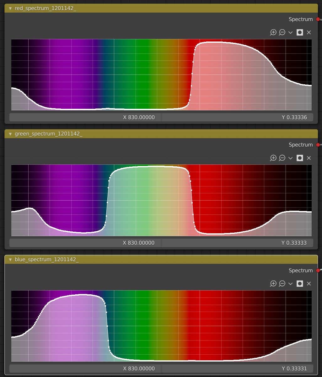
def save_spectra_to_csv(spectra, illuminant_spectrum):
    channels = ['red', 'green', 'blue']
    for i, channel in enumerate(channels):
        filename = f"{channel}_spectrum.csv"

        wl = np.arange(360, 831)
        data = np.column_stack((wl, spectra[:, i]))
        np.savetxt(filename, data,
                   delimiter=",", fmt='%.20E', header=f"wavelength | {channel} spectrum", comments='')
        data = np.column_stack((wl, spectra[:, i] * illuminant_spectrum))
        np.savetxt(f"{filename}_light", data,
                   delimiter=",", fmt='%.20E', header=f"wavelength | {channel} spectrum", comments='')


def main():

    # get the color matching functions and the white point
    cmfs = MSDS_CMFS['CIE 1931 2 Degree Standard Observer']
    d65_spectral = colour.SDS_ILLUMINANTS['D65'].align(cmfs.shape)
    d65_XYZ = colour.sd_to_XYZ(d65_spectral, cmfs=cmfs)
    d65_spectral = colour.SDS_ILLUMINANTS['D65'].align(cmfs.shape) / d65_XYZ[1]  # normalize to Y=1
    d65_XYZ = colour.sd_to_XYZ(d65_spectral, cmfs=cmfs)

    # switch to torch and cuda
    m = torch.tensor(cmfs[:], dtype=FTYPE).cuda()
    d65_spectral = torch.tensor(d65_spectral[:], dtype=FTYPE).cuda()
    d65_XYZ = torch.tensor(d65_XYZ, dtype=FTYPE).cuda()

    okw = xyz_to_oklab(d65_XYZ)  # get the whitepoint in OKLab (for D65 that's basically 1 0 0)

    RGB = torch.tensor(  # whitepoint-agnostic Rec.709 (exact)
        [
            [
                [1664/1245, -2368/3735, -256/1245],
                [286/415, -407/1245, -44/415],
                [26/415, -37/1245, -4/415]
            ],
            [
                [-863/2490, 5011/7470, 37/2490],
                [-863/1245, 5011/3735, 37/1245],
                [-863/7470, 5011/22410, 37/7470]
            ],
            [
                [5/498, -55/1494, 95/498],
                [1/249, -11/747, 19/249],
                [79/1494, -869/4482, 1501/1494]
            ]
        ], dtype=FTYPE).cuda()

    rgb = torch.einsum("...a,a->...", RGB, d65_XYZ).cuda()  # get RGB with the correct whitepoint and primaries

    # define the initial parameters: Red /, Green /\, Blue \
    params = torch.zeros_like(m, dtype=FTYPE).T.cuda()
    params[0] = torch.linspace(-1, 1, steps=params[0].shape[0]).cuda()
    params[1] = torch.linspace(-1, 1, steps=params[0].shape[0]).abs().mul(-1).add(0.5).cuda()
    params[2] = torch.linspace(1, -1, steps=params[2].shape[0]).cuda()
    params = params.requires_grad_(True)

    # pick an optimizer, register parameters, pick hyperparameters
    optimizer = Opt.AdamW(params=(params,), lr=0.001, weight_decay=1/(1 << 64), amsgrad=True)

    SAMPLES: int = 64  # how many spectra to sample each iteration. Will effectively be squared so if 64 then 64² = 4096

    # define the plot settings and update accordingly
    fig, ax = plt.subplots()
    lines = [ax.plot([], [], color=color, label=f'{color}')[0] for color in ['r', 'g', 'b']]
    ax.set_xlim(0, 471)
    ax.set_ylim(0, 1)
    ax.legend()
    plt.ion()
    plt.show()

    def update_plot(plot_spectra) -> None:
        """
        Updates the plot with the latest spectra data.
        """
        for i, line in enumerate(lines):
            line.set_data(range(471), plot_spectra[:, i])
        ax.relim()
        ax.autoscale_view()
        plt.draw()
        plt.pause(0.001)

    def train():
        # sample different colors
        RGB_spectra = params.softmax(dim=0)  # convert the params into the base spectra that sum to 1
        rand_rgb = torch.rand(SAMPLES, 3, dtype=FTYPE).cuda()  # sample {SAMPLES} linear combinations of base spectra
        sample_spectra = (rand_rgb @ RGB_spectra)  # generate the colors
        target_ok = xyz_to_oklab(rand_rgb @ rgb)  # figure out OKLAB coordinates of those target colors

        # generate the spectra corresponding to those colors, as well as higher powers of those spectra
        samples = torch.tensor([sample for _, sample in zip(range(SAMPLES-1), exps)])
        sample_spectra = torch.flatten(torch.stack((sample_spectra, *[sample_spectra**s for s in samples])), end_dim=1)
        xyzs = torch.einsum('...ac,...cb->...ab', sample_spectra * d65_spectral, m)  # multiply by illuminant d65
        oks = xyz_to_oklab(xyzs)  # figure out the OKLab coordinates of the specta

        # calculate losses:
        # square distance between target OKLab coordinates and those calculated for the spectra
        point_loss = N.MSELoss()(oks[:SAMPLES], target_ok)

        # distance from line through OKLab space such that
        rep_rand_ok = target_ok.repeat(repeats=(SAMPLES, 1))
        line_loss = line_dist(okw[1:], rep_rand_ok[:, 1:], oks[:, 1:]).mean()

        tv_loss = (RGB_spectra[..., 1:]-RGB_spectra[..., :-1]).square().sum()

        loss =\
            (
                100000000 * point_loss
                + line_loss
                + tv_loss
            )

        loss.backward()
        optimizer.step()
        optimizer.zero_grad()

        # logging and saving outputs
        latest_spectra = RGB_spectra.T.cpu().detach().numpy()
        latest_loss = loss.item()
        latest_point_loss = point_loss.item()
        latest_line = line_loss.item()
        latest_tv = tv_loss.item()

        return latest_spectra, latest_loss, latest_point_loss, latest_line, latest_tv

    # set up a timer to get regular updates
    iteration = 0
    starttime = time.monotonic()
    curtime = starttime

    while True:  # main training and logging loop
        try:
            spectra, full_loss, ploss, lloss, tvloss = train()
            if time.monotonic() - curtime > 0.25:
                curtime = time.monotonic()
                ips = iteration/(curtime - starttime)
                print(f"i: {iteration}\ti/s: {ips:.3g}\t"
                      f"L: {full_loss:.8E}\t"
                      f"p: {ploss:.8E}\t"
                      f"l: {lloss:.8E}\t"
                      f"tv: {tvloss:.8E}\t"
                      )
                update_plot(spectra)
            iteration += 1

        except KeyboardInterrupt:  # it saves upon cancelling the script (Ctrl + C)
            save_spectra_to_csv(spectra, (100 * d65_spectral).cpu().detach().numpy())
            break


if __name__ == '__main__':
    main()


EDIT 2

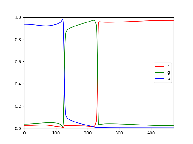
I think I have been overcomplicating things. It turns out if you optimize in OKLab space (rather than XYZ space), you get smooth spectra from literally just directly optimizing the coordinate without any smoothness constraint, and the resulting colors much more strongly correspond to the desired target colors and they perform more strongly in tests overall:


HSV Sweep

current | new

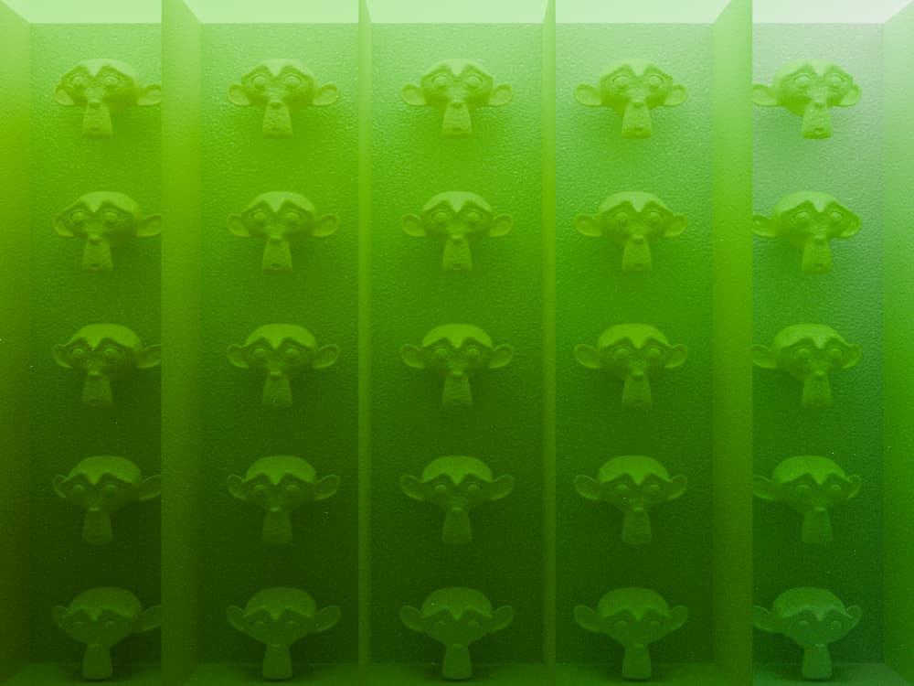
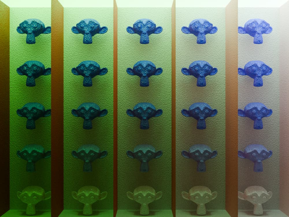
Note the strong purple cast in the blue in the current version. Red also goes slightly purplish.

25 Suzannes


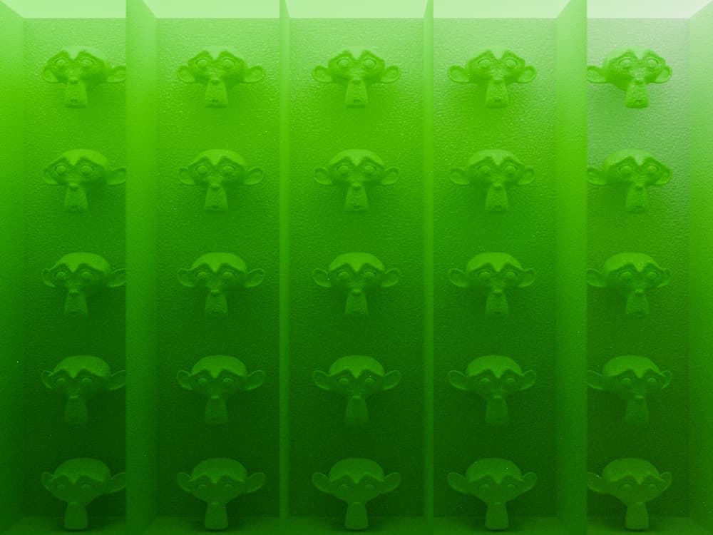
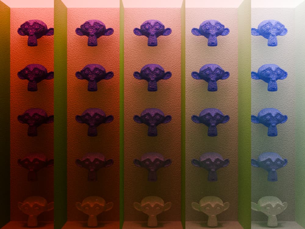
Very strong adherence to constant hue throughout, no purple cast. The bluish cast on the far right of each of these (most noticeable in the all-red version) is due to the D65 whitepoint of the light source while this version of the Spectral Branch actually aims for Illuminant E rendering. AFAIK, that conversion is done through an ad-hoc hack that could be taken out with this approach.

36 Tubes:

One thing this variant doesn’t do is shift blue and yellow to be a bit more pleasant in deeper bounces. But it is closer to the actual RGB values you’d try to obtain.

The spectra:

spectra_optimized_by_OKLab_distance.zip.txt (41.9 KB)

12 Likes